本系列文章配套代码获取有以下两种途径:
-
通过百度网盘获取:
链接:https://pan.baidu.com/s/1jG-rGG4QMuZu0t0kEEl7SA?pwd=mnsj提取码:mnsj
-
前往GitHub获取:
https://github.com/returu/Data_Visualization函数语法:
plt.broken_barh(xranges, yrange, *, data=None, **kwargs)-
xranges: 数组或列表,定义水平断条的x 轴区间,格式为[(x_start1, x_length1), (x_start2, x_length2), ...],其中x_start是区间起始值,x_length是区间长度(非结束值); -
yrange: 元组,定义水平断条的y 轴位置,格式为(y_start, y_height),y_start是条块在 y 轴的起始坐标,y_height是条块的高度(单个类别下所有断条共享同一 y 轴位置); -
data:字典或 DataFrame,允许通过字符串指定数据列; -
**kwargs: 其他绘图参数,如颜色、线宽、透明度、填充图案等。
通过调整这些参数,可以灵活控制水平断条图的视觉效果。
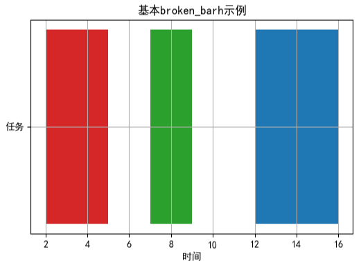
fig, ax = plt.subplots(figsize=(6, 4))

# 绘制三个区间段,分别从x轴的2、7、12位置开始,长度为3、2、4
xranges = [(2, 3), (7, 2), (12, 4)]
yrange = (5, 2)

ax.broken_barh(xranges, yrange, facecolors=('tab:red', 'tab:green', 'tab:blue'))

ax.set_xlabel('时间')
ax.set_yticks([6])
ax.set_yticklabels(['任务'])
ax.set_title('基本broken_barh示例')
ax.grid(True)

plt.show()
可视化结果如下图所示:
使用示例:
-
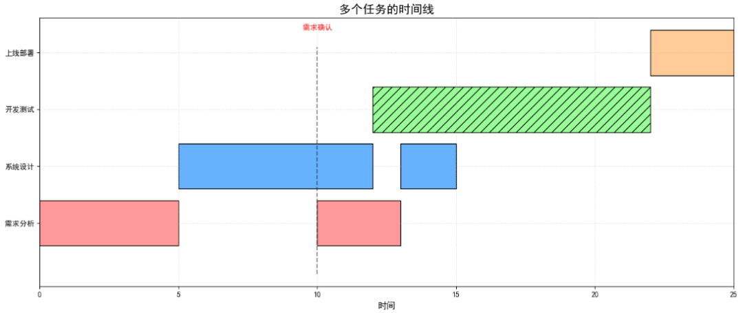
示例1:多个任务的时间线
使用 broken_barh()函数绘制多个任务时间线的核心原理是通过分段区间定义和分层布局,将不同任务的非连续时间段以水平断条形式直观呈现。
import matplotlib.pyplot as plt

# 定义项目阶段数据(名称、时间段、颜色)
phases = [
    {'name': '需求分析', 'ranges': [(0, 5), (10, 3)], 'color': '#FF9999'},
    {'name': '系统设计', 'ranges': [(5, 7), (13, 2)], 'color': '#66B2FF'},
    {'name': '开发测试', 'ranges': [(12, 10)], 'color': '#99FF99'},
    {'name': '上线部署', 'ranges': [(22, 3)], 'color': '#FFCC99'}
]

fig, ax = plt.subplots(figsize=(14, 6))

# 绘制每个阶段
for i, phase in enumerate(phases):
    # 绘制水平断条图
    ax.broken_barh(phase['ranges'], (i + 0.5, 0.8),
                   facecolor=phase['color'], edgecolor='black',
                   hatch='//'if'测试'in phase['name'] else None)  # 测试阶段添加斜线填充

# 设置y轴
ax.set_yticks([i + 0.9 for i in range(len(phases))])
ax.set_yticklabels([phase['name'] for phase in phases])

# 添加里程碑标记
ax.plot([10, 10], [0, len(phases)], 'k--', alpha=0.5)  # 需求分析结束线
ax.text(10, len(phases)+0.3, '需求确认', ha='center', color='red')

ax.set_title('多个任务的时间线', fontsize=16)
ax.set_xlabel('时间', fontsize=12)
ax.set_xlim(0, 25)
plt.grid(True, linestyle=':', alpha=0.5)
plt.tight_layout()
plt.show()
可视化结果如下图所示:
-
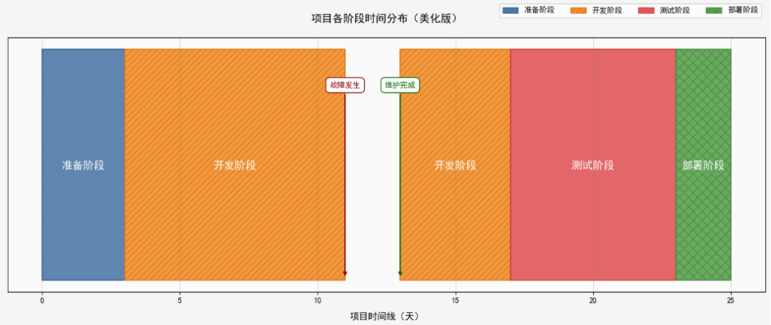
示例2:样式定制与美化
broken_barh()函数提供了细粒度的样式参数,可针对颜色(填充 / 边框、形态(图案 / 线宽)、透明度等维度单独调控,满足个性化设计需求。并根据需要对图表中的其他辅助元素样式进行调整。
from matplotlib.patches import Patch
import matplotlib.pyplot as plt

# 数据准备
phases = {
    '准备阶段': [(0, 3)],
    '开发阶段': [(3, 8), (13, 4)],  # 有中断
    '测试阶段': [(17, 6)],
    '部署阶段': [(23, 2)]
}

# 自定义颜色和样式
colors = ['#4E79A7', '#F28E2B', '#E15759', '#59A14F']
edge_colors = ['#2E5A8A', '#D9781A', '#D13739', '#498D3F']
hatches = ['', '///', '', 'xx']

fig, ax = plt.subplots(figsize=(14, 6), facecolor='#F5F5F5')

# 循环绘制每个阶段的水平断条
for i, (phase, periods) in enumerate(phases.items()):
    ax.broken_barh(
        periods,                # 当前阶段的时间区间列表
        (1, 6),                 # y轴参数:(起始位置, 条块高度),所有阶段在同一水平轨道
        facecolors=colors[i],   # 填充色
        edgecolors=edge_colors[i],  # 边框色
        linewidth=1.5,          # 边框线宽
        alpha=0.9,              # 透明度
        hatch=hatches[i]        # 填充图案
    )

    # 在每个阶段条的中心位置添加阶段名称标签
    for start, duration in periods:
        ax.text(
            start + duration/2,  # 文本x坐标:阶段条的水平中心(起始位置+一半持续时间)
            4,                   # 文本y坐标:阶段条的垂直中心(1+6/2=4)
            phase,               # 显示的文本内容(阶段名称)
            ha='center',         # 水平对齐:居中
            va='center',         # 垂直对齐:居中
            fontsize=14,         # 字体大小
            fontweight='bold',   # 字体粗细
            color='white'        # 文本颜色
        )

# 添加事件标记
ax.annotate(
    '故障发生',
    xy=(11, 1),  # 箭头指向的位置
    xytext=(11, 6),  # 文本位置
    arrowprops=dict(
        arrowstyle='->',
        color='darkred',
        linewidth=1.5,
        shrinkB=5  # 箭头与目标点的距离
    ),
    ha='center',
    color='darkred',
    fontweight='bold',
    bbox=dict(facecolor='white', edgecolor='darkred', pad=3, boxstyle='round,pad=0.5')  # 文本背景框
)
ax.annotate(
    '维护完成',
    xy=(13, 1),  # 箭头指向的位置
    xytext=(13, 6),  # 文本位置
    arrowprops=dict(
        arrowstyle='->',
        color='darkgreen',
        linewidth=1.5,
        shrinkB=5
    ),
    ha='center',
    color='darkgreen',
    fontweight='bold',
    bbox=dict(facecolor='white', edgecolor='darkgreen', pad=3, boxstyle='round,pad=0.5')
)


# 创建图例
legend_elements = [Patch(facecolor=colors[i], edgecolor=edge_colors[i],
                         label=phase, hatch=hatches[i])
                   for i, phase in enumerate(phases.keys())]
ax.legend(handles=legend_elements, loc='upper right',
          bbox_to_anchor=(1, 1.15), ncol=4)

# 美化图表
ax.set_xlabel('项目时间线(天)', fontsize=12, labelpad=10)
ax.set_title('项目各阶段时间分布(美化版)',
             fontsize=14, pad=20, fontweight='bold')
ax.grid(True, linestyle='--', alpha=0.4, color='gray')
ax.set_facecolor('#FAFAFA')

# 隐藏y轴刻度
ax.set_yticks([])
plt.tight_layout()
plt.show()
可视化结果如下图所示:
更多内容可以前往官网查看:
https://matplotlib.org/stable/


本篇文章来源于微信公众号: 码农设计师